Autoscaling with Grafana and Prometheus

In the last 12 months, we released several fundamental services that greatly simplify the deployment of larger architectures. While each of the building blocks on its own is not enough to solve all problems you may be facing, they can and should be used together to build up your own infrastructure efficiently.

In this article, we will demonstrate how those building blocks, such as the Network Load Balancer and Instance Pools, can be used together to achieve an automatically scaling and highly available deployment.

For the purposes of this example, each member of the Instance Pool will run a webserver to serve web content and a Prometheus node exporter to gather metrics.

A central Prometheus instance will collect the metrics, pass them to Grafana, and use a simple utility to scale the Instance Pool on demand based on the selected metrics. The Load Balancer will scale accordingly, distributing traffic to all underlying instances in the Instance Pool.

Setting Up the Instance Pool

As a first step, we need a running Instance Pool to run our web application.

We will intentionally use a very small machine for the demo, and we will scale the Pool based on CPU load. This is an arbitrary choice for demo purposes, but you could use any type of machine and metrics.

To simulate the needed metrics to trigger the scale, we will run a tiny webserver specifically written to generate CPU load for every request.

Along the application we need to install the Prometheus node exporter that will be used to gather metrics from each instance.

Using an Instance Pool, we need a way to ensure that new Instances added to the pool will have all the required packages and setup needed to work as their siblings. There are mainly two ways to achieve this goal:

1. Scripting any installation step in the User Data
2. Using a Custom Template

In our case. we will use a simple script that installs Docker and then launches the load generator and node exporter services.

If you want to follow along, please grab the script from GitHub and save it as userdata.sh on your computer.

Apart from the above, the rest of the Instance Pool can be pretty much left on the standard settings. The only exception are the security groups, which we have to adjust to our needs. We should allow in port 8080 for the web traffic from 0.0.0.0/0 and ports 3000 and 9090 from only our IP for Grafana and Prometheus. Inside the security group, all traffic should be allowed.

We will use the exo command line client command-line utility to create the needed resources. Of course, every action can also be performed through our web portal if you feel more comfortable with a GUI.

Let’s start by creating the following security group and rules:

exo firewall create autoscaling
exo firewall add autoscaling --protocol tcp --port 22
exo firewall add autoscaling --protocol tcp --port 8080-8080
exo firewall add autoscaling --protocol tcp --port 3000-3000
exo firewall add autoscaling --protocol tcp --port 9090-9090
exo firewall add autoscaling --protocol tcp --port 1-65535 -s autoscaling
exo firewall add autoscaling --protocol udp --port 1-65535 -s autoscaling
exo firewall add autoscaling --protocol icmp -s autoscaling

You can then create the Instance Pool with the previously downloaded userdata.sh file:

INSTANCEPOOL_ID=$(exo instancepool create autoscaling \
    --service-offering Tiny \
    --template "Linux Ubuntu 20.04 LTS 64-bit" \
    --zone at-vie-1 \
    --security-group autoscaling \
    --cloud-init userdata.sh \
    --disk 10 \
    --size 2 \
    --output-template '{{ .ID }}')

After a few minutes, we can query the instance pool and see that the two instances have been launched:

# exo instancepool show autoscaling
┼──────────────────┼──────────────────────────────────────┼
│ ID               │ 5cb6e895-e7a5-03fd-95ab-b0f66871eefb │
│ Name             │ autoscaling                          │
│ Description      │                                      │
│ Service Offering │ Tiny                                 │
│ Template         │ Linux Ubuntu 20.04 LTS 64-bit        │
│ Zone             │ at-vie-1                             │
│ Security Groups  │ autoscaling                          │
│ Private Networks │ n/a                                  │
│ SSH Key          │                                      │
│ Size             │ 2                                    │
│ Disk Size        │ 10 GiB                               │
│ State            │ running                              │
│ Instances        │ pool-5cb6e-utogc                     │
│                  │ pool-5cb6e-daqxq                     │
┼──────────────────┼──────────────────────────────────────┼

Our instances are now running, and they are in the process of installing Docker.

Setting Up the Network Load Balancer

While our Docker installation is running on each pool member, we can create a new load balancer, and then add a new service with the following settings:

• Name: HTTP
• Instance Pool: select the previously created Instance Pool
• Strategy: Round Robin
• Protocol: TCP
• Service Port: 80
• Target Port: 8080
• Health Check Protocol: HTTP
• Health Heck Port: 8080
• Health Check Path: /health

exo nlb create autoscaling -z at-vie-1
exo nlb service add autoscaling HTTP \
    --description HTTP \
    --healthcheck-mode http \
    --healthcheck-uri /health \
    --instance-pool-id "${INSTANCEPOOL_ID}" \
    --port 80 \
    --target-port 8080 \
    --zone at-vie-1

While we wait for the NLB service to bootstrap the health-check, we can retrieve the IP address of our load balancer and use it to print out the correct address for the load generating website:

NLB_IP=$(exo nlb show autoscaling --output-template '{{ .IPAddress }}')
echo "http://${NLB_IP}/load"

By pasting the address in a browser tab, the browser should load for a while and then return with a simple message saying that the load generation is complete. If it doesn’t immediately work, ensure that the health-check of our service reports a “success” status:

exo nlb service show autoscaling HTTP --output-template "{{ .HealthcheckStatus }}"

We now have a service that can be scaled up and down manually. We can also easily generate a heavy load on it simply by opening the load-generating URL above, so it should be ideal for testing.

Starting a monitoring server

For the next step we will need to start a monitoring server that will run Prometheus, Grafana, as well as two custom utilities for service discovery and the actual autoscaling.

The monitoring server will make extensive use of Docker, so we will use a Docker installation script to be used with cloud init. Please download the script and save it as install-docker.sh. Once we have the script locally, we can start the instance:

exo vm create autoscaling-monitor \
    -o micro \
    -f install-docker.sh \
    -t "Linux Ubuntu 20.04 LTS 64-bit" \
    -s autoscaling
    -z at-vie-1

Let’s note down the IP of the monitoring server for later reference:

MONITORING_IP=$(exo vm show autoscaling-monitor --output-template "{{ .IPAddress }}")
echo $MONITORING_IP

You can then SSH into the new monitoring instance with the following command:

exo ssh autoscaling-monitor

All subsequent commands should be launched in this SSH session.

Gathering Metrics With Prometheus

Before we dive into automating the scaling operations, we have to be able to collect some metric to make decisions upon.

Prometheus is uniquely suited for this task because it can gather metrics from a dynamic number of hosts, adapting to our pool size. The process of letting Prometheus know the list of IP addresses it needs to collect metrics from is called service discovery.

Implementing Service Discovery

To add Exoscale service discovery to Prometheus, we need to produce a file in the following format for the file_sd_config option:

[
  {
    "targets": [ "IP 1", "IP 2", "..." ],
    "labels": {}
  }
]

A simple option to generate such a file could be to write a simple bash script and launch it from a cron job. This would refresh the file every minute.

A cleaner and more performant solution would be to write a small agent that will query the Exoscale API every few seconds (much faster than a cron-based solution could) and output a file in the above format.

Exoscale provides different language bindings to ease the creation of such custom tools. In this example, we will be using Go and the related Go library for Exoscale, but a Python library exists too, and the community has added a large number of libraries for other languages too.

You can find a working example of a service discovery generator service here. Its usage is pretty straightforward: by instantiating a new egoscale.Client we go and fetch the desired pool via the API, and generate the file.

To start the service on our monitoring server we first need to create a folder to share the aforementioned file in:

mkdir -p /srv/service-discovery/
chmod a+rwx /srv/service-discovery/

Next, we will start the service discovery agent, substituting out API key and secret, as well as the instance pool ID.

sudo docker run \
    -d \
    -v /srv/service-discovery:/var/run/prometheus-sd-exoscale-instance-pools \
    janoszen/prometheus-sd-exoscale-instance-pools:1.0.0 \
    --exoscale-api-key EXO... \
    --exoscale-api-secret ... \
    --exoscale-zone-id 4da1b188-dcd6-4ff5-b7fd-bde984055548 \
    --instance-pool-id ...

Running Prometheus

Now that we have the service discovery up and running, we can launch Prometheus proper. First, we create the prometheus.yml file in /etc/prometheus that we will mount in the Prometheus container:

global:
  scrape_interval: 15s
scrape_configs:
  - job_name: ’prometheus’
    static_configs:
      - targets: [’localhost:9090’]
  - job_name: ’exoscale’
    file_sd_configs:
      - files:
          - /srv/service-discovery/config.json
        refresh_interval: 10s

Then we can start Prometheus:

sudo docker run -d \
    -p 9090:9090\
    -v /etc/prometheus/prometheus.yml:/etc/prometheus/prometheus.yml \
    -v /srv/service-discovery/:/srv/service-discovery/ \
    prom/prometheus

Let’s exit the SSH connection with exit, and run the following command referencing the MONITORING_IP we have previously saved:

echo "http://${MONITORING_IP}:9090/"

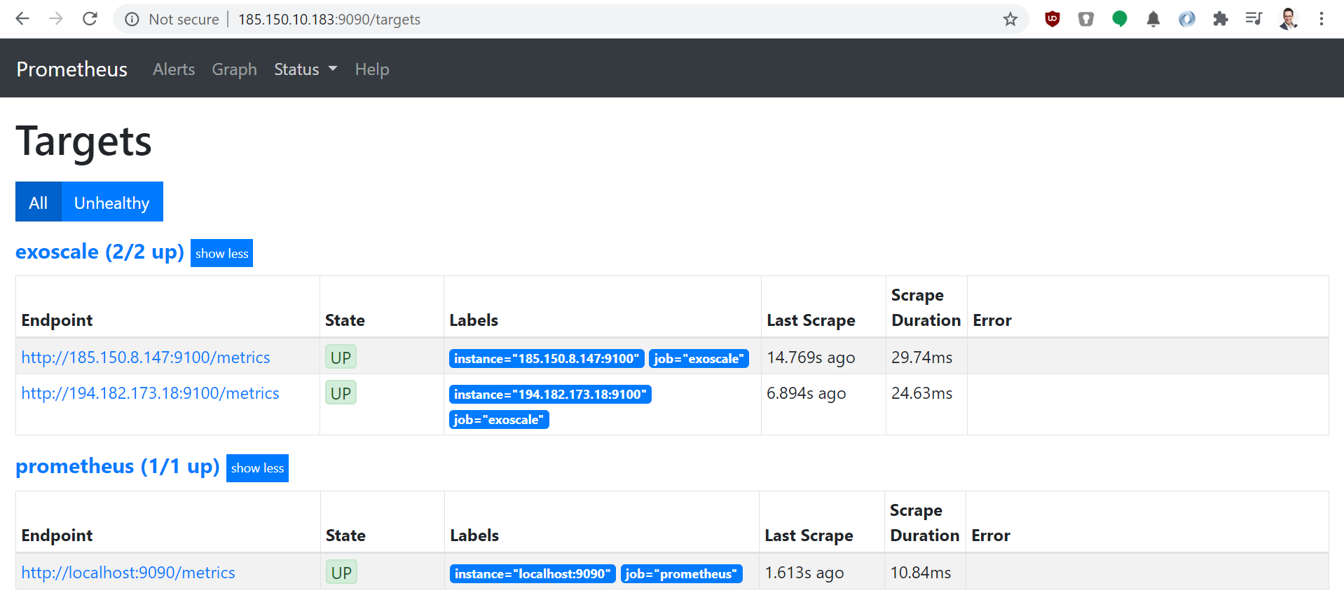
This will print out the address of the Prometheus server. The Status → Target menu should give us the two instances currently running in the Instance Pool:

Setting up Grafana

After logging back into the monitoring server via SSH with exo ssh autoscaling-monitor we can set up Grafana.

While the Prometheus alert manager would probably be more than enough to drive the actual autoscaling behavior, Grafana however, will provide us a graphical overview of what is going on, and let us configure the automatic scaling from a friendly web interface.

So, let’s start Grafana with Docker:

sudo docker run -d \
    -p 3000:3000 \
    grafana/grafana

That’s it, you can drop out of the SSH connection with exit and use the following command to get the Grafana URL:

echo "http://${MONITORING_IP}:3000/"

Copy the link into a browser, and you should see the Grafana dashboard. The default username is admin, and the password is also admin. Grafana will prompt us to change this immediately.

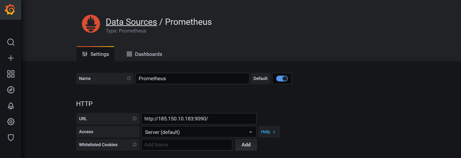
Now we can select Configuration → Data sources on the left side, add a Prometheus data source and use the monitoring server’s public IP to fetch the data from Prometheus:

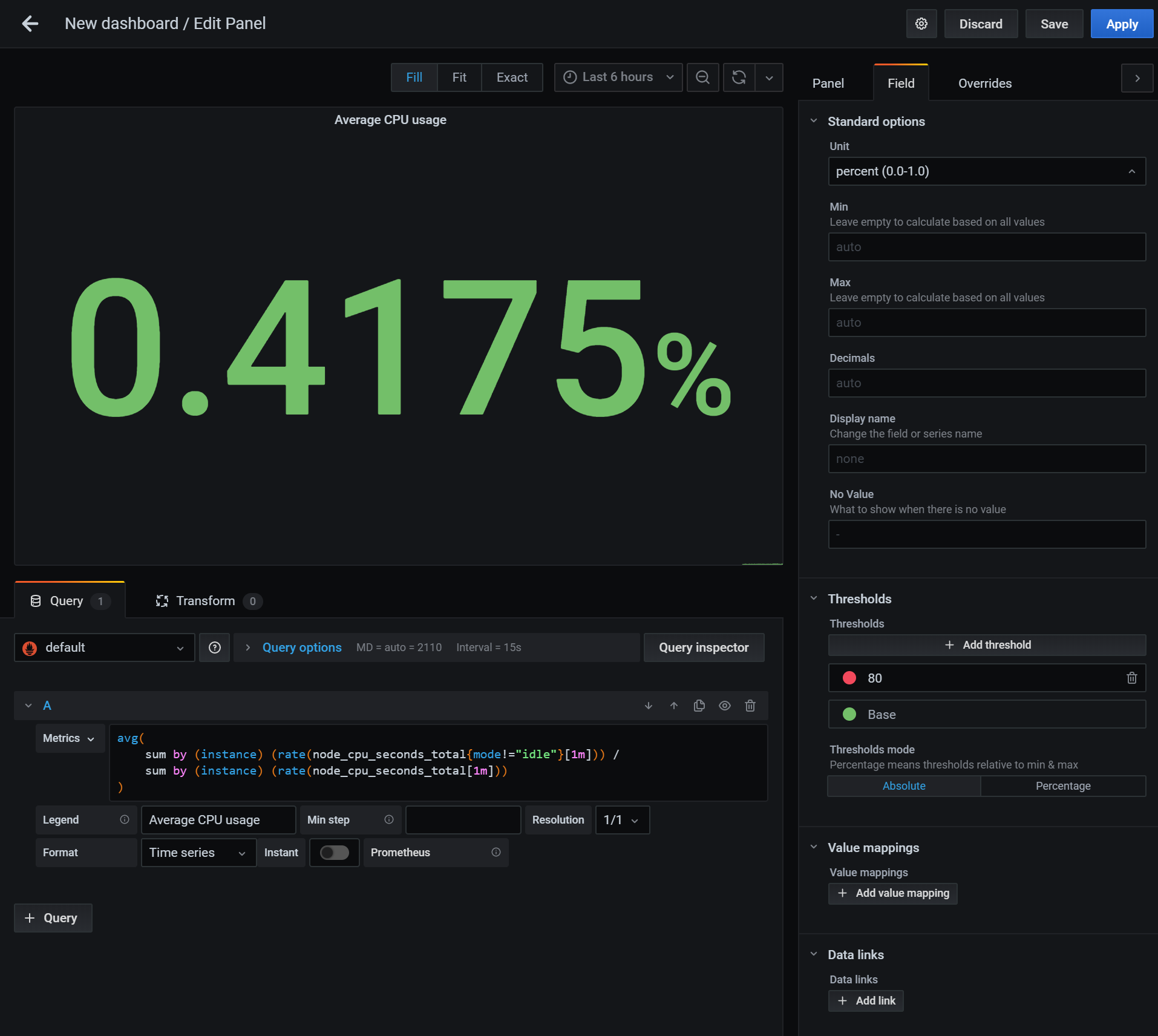
Next, we can set up a new dashboard by clicking + sign on the left side. We can then create a panel to display our CPU usage. We do this by adding the following formula to the Metrics field:

avg(
    sum by (instance) (rate(node_cpu_seconds_total{mode!="idle"}[1m])) /
    sum by (instance) (rate(node_cpu_seconds_total[1m]))
)

We can also change the display options on the right side:

By hitting our load balancer IP, we can verify if the CPU metrics rise as expected. ab is a server benchmarking tool that will let us easily do concurrent calls. (Note that you need to replace ${NLB_IP} by hand if you are not running this on your own machine.)

ab -c 4 -n 1000 http://${NLB_IP}/load

We should see a sharp spike in CPU usage once we hit the top right “refresh” button in Grafana. At this point, make sure to save your dashboard in Grafana.

Configuring Grafana for Autoscaling

The next step will be to configure Grafana for autoscaling. For that, we will set up one alert channel for scaling up, and one for scaling down.

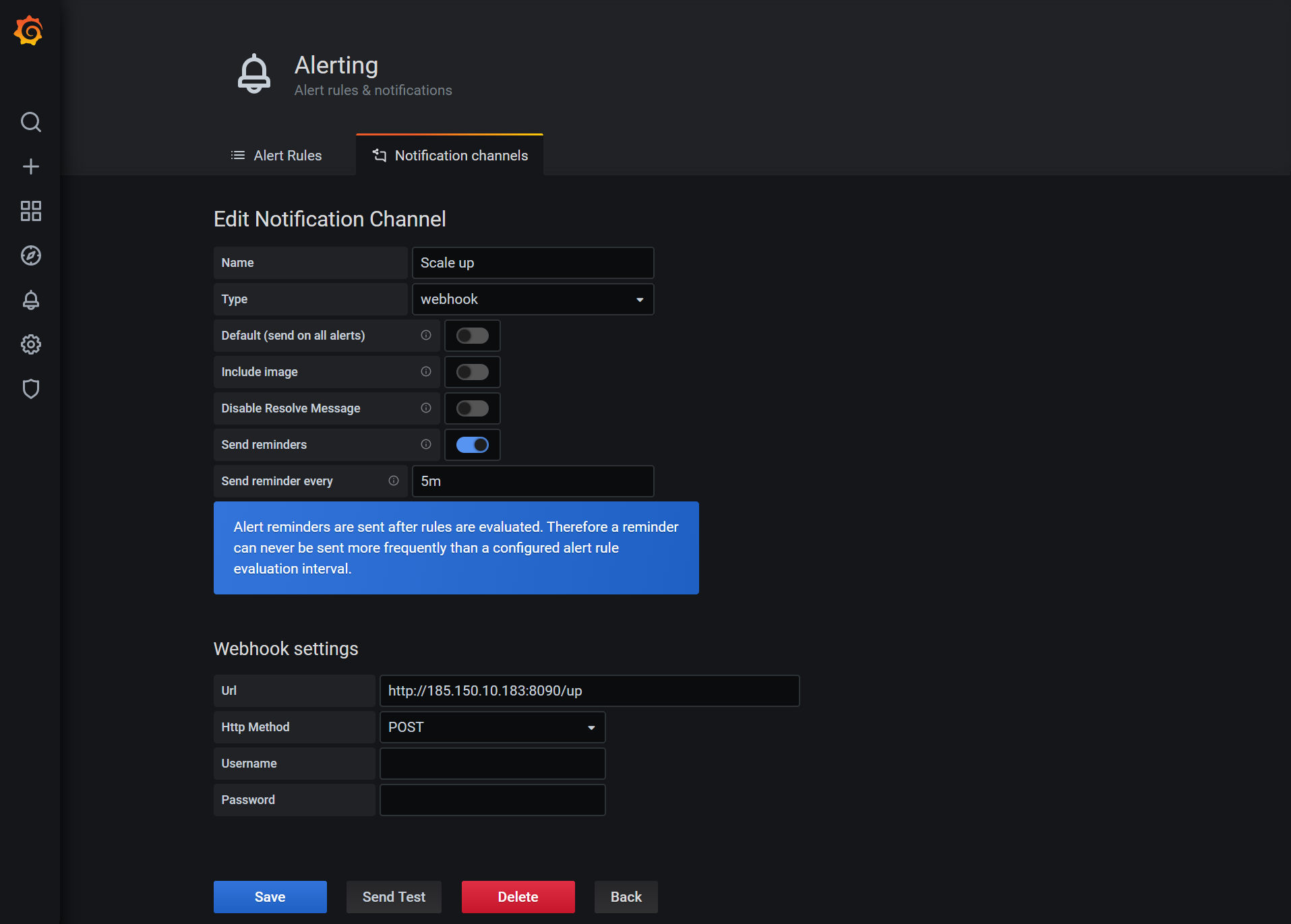
Click “Alerting” on the left menu and then set up a new alert channel. We will name this channel Scale up and select the webhook type. As the URL we will add the monitoring server’s IP address with the port number 8090 and the path /up:

We should also set the “Send reminders” option at this point, so we repeatedly scale up if the CPU usage is still high. The autoscaler itself will limit the size of the Instance Pool to a minimum and maximum, avoiding an infinite scaling loop.

Now, repeat the process with the down part.

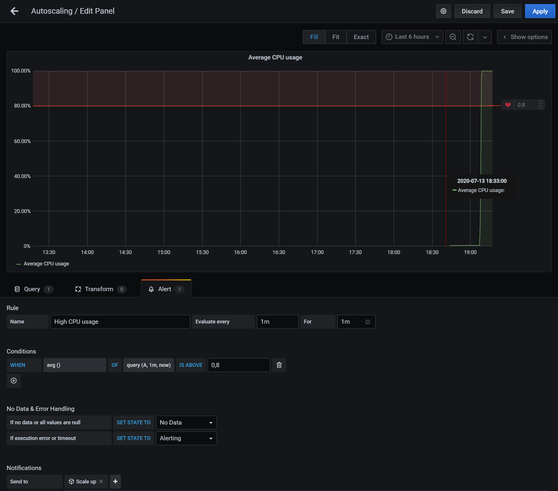
Once that’s done, we can head back to our dashboard and change the CPU usage monitoring to add an alert when the average CPU usage over one minute is over 80%. We should set the notification to use the Scale up channel.

Note: The alerting option is not available on all visualization types. Make sure to create a “graph” type.

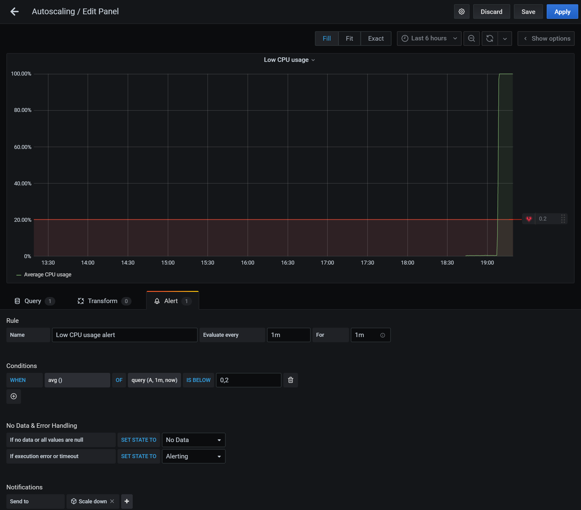
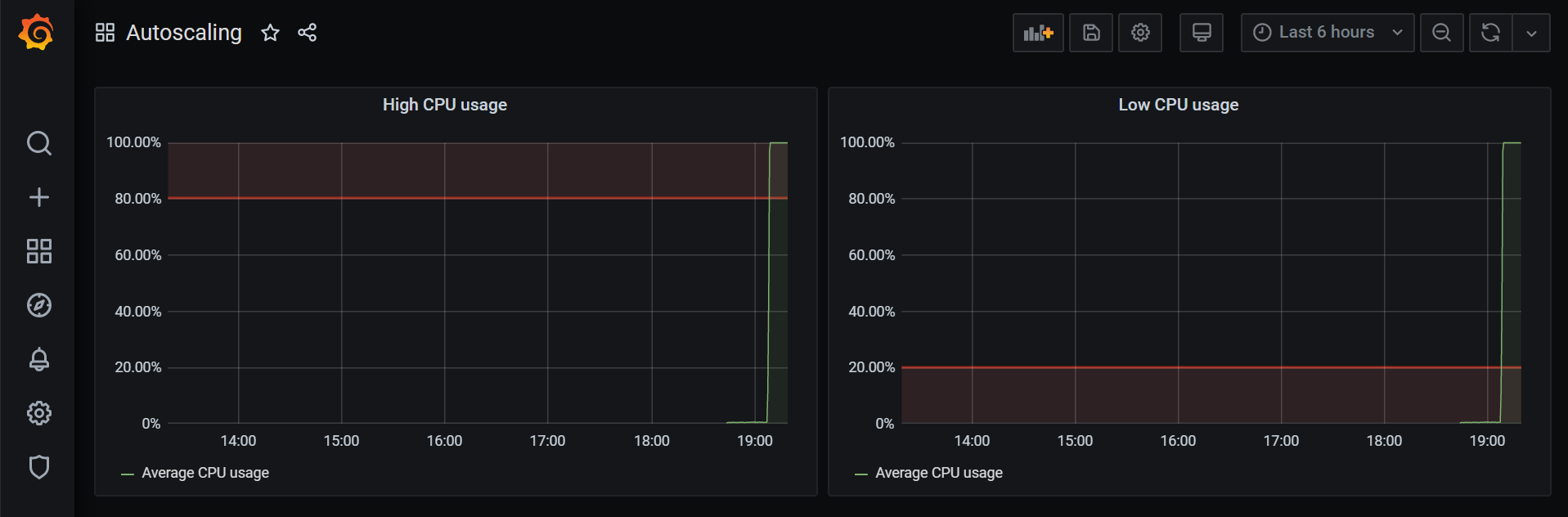
Let’s save the dashboard and duplicate the graph, this time naming it “Low CPU usage” and adding an alert when the CPU usage is below 20%:

The final dashboard should look something like this:

Implementing the Autoscaler

There is one important piece missing from the puzzle: the autoscaler itself. Grafana will send webhooks to port 8090 every 5 minutes when the CPU usage breaches the high or low watermark. We will have to handle these webhooks with a custom application.

As before, we can use Exoscale language bindings to implement it, and we’ll use Go once more in our example. You can find the source code of the full sample implementation on GitHub.

Our software’s role is to accept HTTP requests from Grafana when the CPU usage is too high, or too low, and scale the Instance Pool accordingly. The main function sets up the webserver and defines the required endpoints to scale /up and /down:

func main() {
    //...
    http.HandleFunc("/up", handler.up)
    http.HandleFunc("/down", handler.down)
    err = http.ListenAndServe(":8090", nil)
    if err != nil {
        log.Fatalf("failed to launch webserver (%v)", err)
    }
}

We can then implement the hooks for the /up and /down URLs like so:

func (handler *requestHandler) up(_ http.ResponseWriter, _ *http.Request) {
    instancePool := handler.getInstancePool()
    if instancePool == nil {
        // Instance pool not found, try next round
        return
    }
    if instancePool.Size <= handler.maxPoolSize {
        handler.scaleInstancePool(instancePool.Size + 1)
    }
}

As you can see, the maxPoolSize restricts the maximum Pool size to a preconfigured limit. A similar logic can be applied to the /down handler. The getInstancePool and scaleInstancePool functions will take care of calling the appropriate APIs endpoint to resize the pool:

func (handler *requestHandler) scaleInstancePool(size int) {
    ctx := context.Background()
    resp, err := handler.client.RequestWithContext(ctx, egoscale.ScaleInstancePool{
        ZoneID: handler.zoneId,
        ID:     handler.poolId,
        Size:   size,
    })

    ...
}

Whether you compiled and packaged the source code, or simply downloaded it from GitHub, is now time to fire it up on the monitoring server:

sudo docker run -d \
    -p 8090:8090 \
    janoszen/exoscale-grafana-autoscaler:1.0.2 \
    --exoscale-api-key EXO... \
    --exoscale-api-secret ... \
    --exoscale-zone-id 4da1b188-dcd6-4ff5-b7fd-bde984055548 \
    --instance-pool-id ...

If we run a load test with ab as we did previously on our setup we should see something like this:

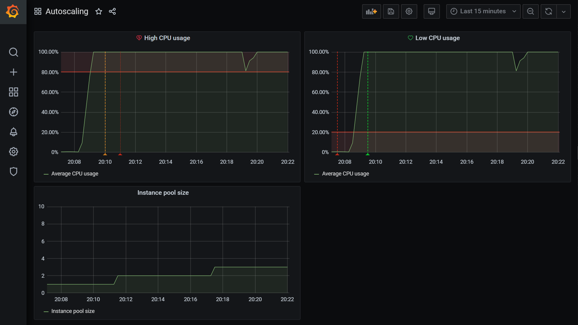
Now all that’s left is to fine-tune the setup to our needs. Keep in mind that our load generating server is artificially slow, so the values provided in this example are going to be close to what you need for a real-life scenario.

Autoscaling in the Real World

We ended up with a prototype of an automated and scalable infrastructure that can react to external conditions and serve in HA fashion any application you may run on it.

A real-world implementation would take several additional steps to be fully implemented, for example, taking advantage of configuration management tools such as Terraform. You may also want to put in backups, redundancy, hardening your setup from a security and stability perspective.

But the seed idea the article wants to transmit is here: understanding APIs and tools gives you the control to implement whatever you need with a significant amount of flexibility. You can react to the particular needs of your business with the help of the cloud building blocks we provide, open-source tools such as Grafana, Prometheus, and just a little bit of a glue layer.