From Commercial API to Sovereign Infrastructure: A Practical Guide to LLM Workload Migration
 Paul Habfast
In January 2026, a software company received a routine notification from their cloud AI provider: the model powering their production pipeline was being deprecated. No migration path, no extended support window, no negotiation. The model that their extraction logic, prompts, and evaluation suite had been built around was simply going away, and the “newer alternatives” were not producing satisfactory results.
At this point, this story is a predictable one. The risk scenario should have been assessed and planned for.
That incident crystallized a question many engineering teams are quietly sitting with: how dependent are we on infrastructure we don’t control? Not just in terms of uptime or API rate limits, but in the deeper sense: who owns and runs the model weights, who can read the traffic, who decides when the service changes?
This post is a practitioner’s guide to answering that question in practice. It is drawn from a collaborative R&D project: the CIEL project, a partnership between Recarta (a Swiss proptech company), HEIG-VD/IICT, SDSC, and Exoscale, that migrated a real, production-grade document intelligence workload off commercial LLM APIs and onto an LLM hosted on sovereign infrastructure. We will share what worked, what didn’t, and the decision-making framework that guided each step.
1. Defining Sovereignty: It’s a Spectrum
The word “sovereign” gets used loosely. Before you can migrate toward it, you need to be precise about what you’re targeting.
There are, practically speaking, three tiers of sovereignty for LLM workloads:
| Tier | Example | Data residency | Control over model | Verdict |
|---|---|---|---|---|
| Public API | OpenAI.com, Anthropic | Data leaves your jurisdiction | None | Not sovereign |
| Private API on hyperscaler | Azure OpenAI in EU region | Physically in EU/CH, but… | None | Partial: see below |
| Dedicated deployment on EU cloud | Exoscale (CH/AT/DE/HR zones) | Fully within jurisdiction | Complete | Fully sovereign |
The middle tier deserves particular attention, because it is where a lot of teams believe they have solved the problem when they haven’t. A model running on Azure in a European datacenter is still operated by a US company. Under the CLOUD Act, US authorities can compel US-headquartered providers to disclose data held on their infrastructure anywhere in the world, regardless of the physical location of the servers. This is a legal reality that some regulated industries (finance, healthcare, legal, real estate) cannot afford to ignore.
Full sovereignty, in a meaningful sense, requires:
- Data processing within EU/CH jurisdiction, on infrastructure operated by a European entity under European law.
- No third-country touchpoint at any stage of the pipeline: not in the inference call, not in the model weight storage, not in the logging infrastructure.
- Control over the model version. Meaning no provider can silently alter, retrain, or retire the model you are running in production. You’re also at the mercy of performance decreases because you don’t control the backend lifecycle. Anthropic’s own April 2026 postmortem is a good illustration: a handful of behind-the-scenes changes (a lowered default reasoning effort, a cached-reasoning bug, and a system prompt tweak) quietly degraded Claude’s quality before they were spotted and rolled back.
- Control over the model pricing and availability. We have seen model providers (such as Anthropic) vary the API price of their models, and filter out some specific usages (with OpenClaw)
Once you know where on this spectrum you need to land, the migration path becomes much clearer.
2. Before You Touch Infrastructure: Build Your Evaluation Set
CIEL is a document-intelligence pipeline. It takes a business document and returns the content as a structured JSON object that follows a fixed schema. Every choice further down in this guide from the model to the chunking to the serving setup exists to do that one thing well. And doing it well first requires a way to measure whether the extraction is actually any good, which is what this section is about. This is the section most migration guides skip, and it is the most important one.
The single biggest factor in the success of the CIEL project was not the choice of model, the inference engine, or the deployment zone. It was the decision, made early and held to consistently, to build a curated, ground-truth evaluation set before doing anything else. Everything that followed flowed naturally from that foundation. Without it, the project would have been navigating blind: unable to compare models objectively, to measure the impact of prompt changes or to know whether a new configuration was an improvement or a performance decrease.
If there is only one thing you take away from this article, it should be that the most impactful thing you can do is to build the evaluation set first.
2.1 What the evaluation set is
An evaluation set is a collection of input documents paired with their expected outputs which represents the ground truth that your extraction pipeline should reproduce. In the CIEL project, this meant real documents (lease contracts, renovation quotes, work orders) paired with manually validated JSON extractions representing exactly what the system should produce.
The final repository contained 54 extraction test documents in French and 37 in German, each with:
- The input document (a representative example of that document type)
- The golden answer (the expected structured JSON, validated by domain experts)
- Metadata including document type, language, and relevant extraction parameters
To give a sense of scale: the test set works out to roughly 1.8 million input tokens and 40,000 individual output field checks. Every one of those 40,000 checks was validated by hand. That was a significant amount of work. It was also the investment that paid for every other decision in the project.
2.2 Why to build it before anything else
When you are migrating from a commercial LLM to an open-weight alternative, you will face a rapid succession of decisions: which model to shortlist, which output format to use, whether to fine-tune, how to set your context window, whether chunking hurts quality. Every one of these decisions benefits from having a concrete, objective answer to the question: is this configuration better or worse than what came before?
In practice, having the evaluation set available from the start meant that:
- Model benchmarking was fast and credible. When evaluating 16 candidate models, running each through the same 91 test cases and comparing mean similarity scores took hours, not weeks of qualitative assessment.
- Prompt engineering became iterative rather than speculative. Every change to the system prompt, few-shot examples, or output schema could be validated immediately against the ground truth.
- Infrastructure decisions were grounded in data. The question “does chunking hurt quality?” was answered with a measured difference in similarity score (roughly 0.05–0.10, ie significant).
- Performance decreases were caught automatically. When a new model version or prompt update degraded performance, the evaluation pipeline flagged it before it reached production.
2.3 What makes a good evaluation set
Size. Aim for 20-50 examples minimum. Below that, variance in individual test cases makes aggregate scores noisy. Above 200, the marginal cost of maintenance starts to outweigh the benefit. The CIEL project settled on around 90 examples across two languages, which was enough to produce stable, statistically meaningful scores.
Representativeness. Cover your full distribution of document types. Include short documents (2 pages) and long ones (300+ pages). Include multilingual content if that is part of your production workload. Include edge cases: documents with dense tables, missing fields, unusual formatting, or atypical structure. The failure modes you don’t test for are the ones that will find you in production.
Ground truth quality. The golden answers need to be correct. This sounds obvious, but it is the hardest part. Domain expert validation takes time. In the CIEL project, initial golden answers were generated by the best available model (GPT-4o at the time) and then manually reviewed and corrected by the team. The review pass is not optional: model-generated pseudo-labels will subtly favour the model that generated them, corrupting your comparative benchmarks.
Versioning. Keep the evaluation set in version control alongside your code. When you add new test cases, tag the set version. When you compare two model configurations, ensure they were evaluated against the same set version. Mixing evaluation set versions is a surprisingly common source of spurious “improvements.”
Living maintenance. Treat the evaluation set as a product, not an artifact. When a customer reports a failure mode you hadn’t seen, add it to the set. When you extend to a new document type, add representative examples before writing a line of code. The set should grow as your production distribution grows.
2.4 How to build it iteratively
You do not need to build the full evaluation set before starting any other work. A practical approach that worked well in this project:
- Start with 5–10 documents per document type. Set 3 aside as few-shot examples for prompting; use the remaining 2+ as initial test cases.
- Run your best available model (even a commercial one) on the test cases. Manually review the outputs and correct them to produce your first golden answers.
- Add new edge cases. As you encounter new problematic cases, add them to the test set immediately, with verified golden answers.
- Run the full evaluation suite on every meaningful change. Model swap, prompt update, schema change, chunking strategy adjustment or any other change can then be mapped to an improvement or degradation.
Avoid skipping the evaluation run when you’re in a hurry. That is precisely when performance decreases slip through.
2.5 Scoring: what to measure
A binary “correct/incorrect” metric is too coarse for structured extraction. Most fields are partially correct: the right value with a minor formatting difference, or an address missing a postal code. The CIEL project used a continuous similarity score based on Levenshtein distance, which gives credit for partial matches and is sensitive to the kinds of variation (abbreviations, spacing, number formatting) that are common in real documents.
For structured outputs, the scoring needs to handle:
- Nested objects score each sub-object independently and aggregate.
- Lists score in an order-insensitive way; a correctly extracted set of line items should score the same regardless of the order they were extracted.
- Missing and extra fields penalize both false negatives (missed extraction) and false positives (hallucinated content) equally, with a score of 0 for each.
- Weighting decide whether a building object and a 200-line quote content block should contribute equally to the final score (object-based weighting) or whether larger content blocks should have more influence (volume-based weighting). Both are useful for different diagnostic purposes.
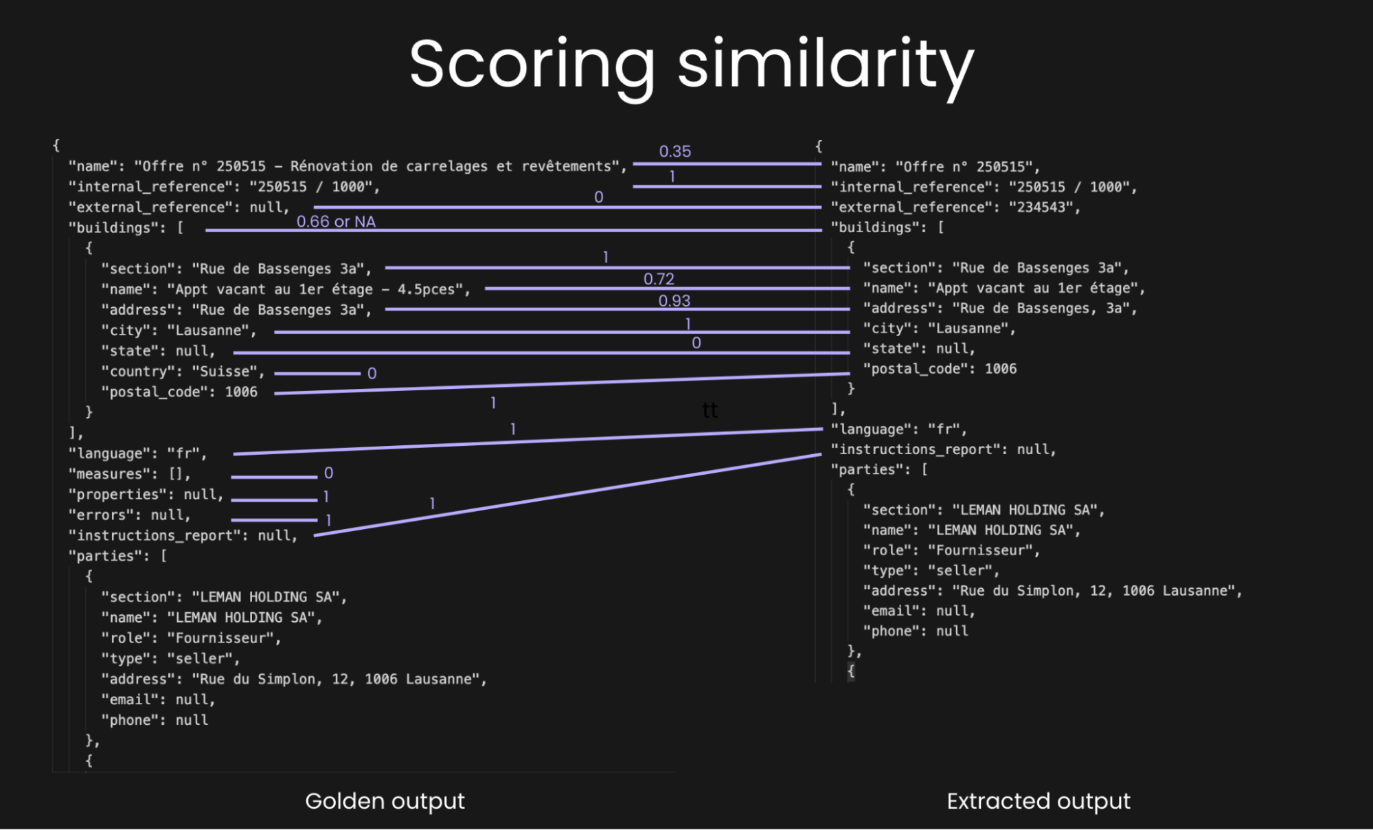
Field-level similarity scoring: each field is scored independently using string similarity, enabling partial credit and fine-grained diagnostics.
The three dimensions worth tracking across every evaluation run are similarity score (accuracy), duration (wall-clock time to process a document), and token usage (input + output tokens per extraction). Together, these give you the accuracy/cost/speed trade-off surface you need to make informed infrastructure decisions.
2.6 Observability: instrument your pipeline before you migrate
One more thing that pays for itself many times over: before migrating off your commercial API, instrument your existing pipeline with an observability tool. In the CIEL project, Phoenix was used to trace every LLM call, logging the full prompt (system + user), the raw output, token counts, latency, and retry history.
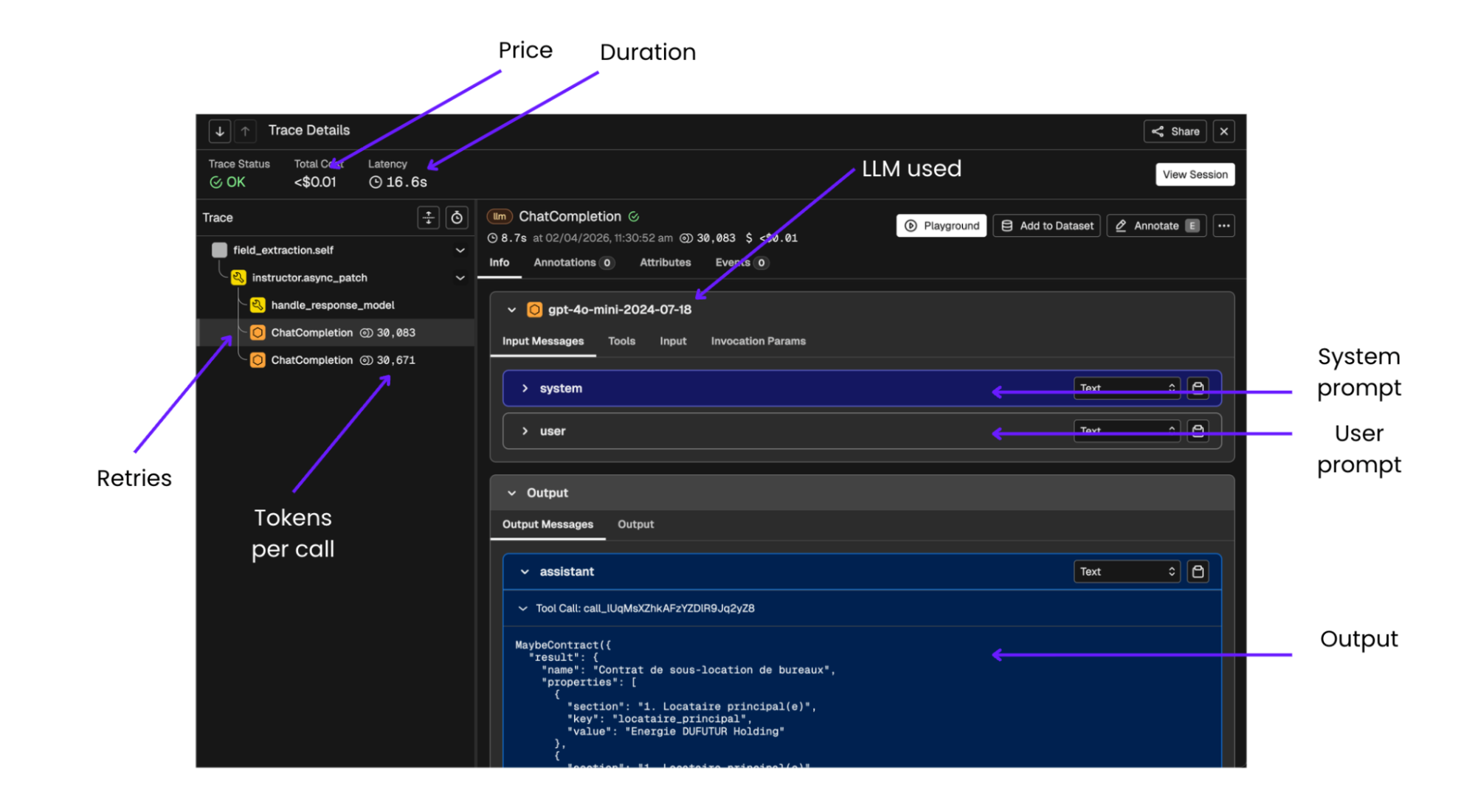
Phoenix trace view: every LLM call is logged with its full prompt, output, token usage, latency, and retry history, essential for baseline measurement and post-migration comparison.
This does two things. First, it gives you baseline numbers such as actual token distributions, latency and retry rates that you will need to evaluate open-weight alternatives fairly. Second, it makes debugging dramatically faster when something goes wrong after migration.
Phoenix is based on OpenTelemetry and is incredibly quick and easy to setup, configure and integrate into most AI pipelines.
3. Model Selection: Open-Weight Is No Longer a Compromise
The assumption that open-weight models sit meaningfully below frontier commercial models does not hold any more for structured extraction. Our experience shows that this was true in 2024 but does not hold anymore.
3.1 The benchmark landscape has shifted
In the CIEL project, 16 open-weight and proprietary models were evaluated on real extraction tasks using the evaluation framework described in Section 2. The proprietary model (GPT-4.1-mini) served as the baseline, as it had been the production model for the commercial pipeline.
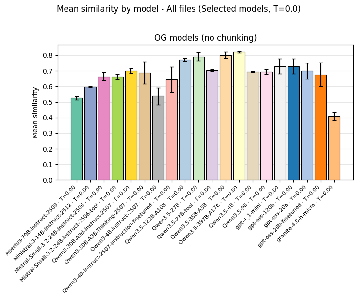
Zero-shot benchmark across 16 models on real extraction tasks. The Qwen3.5 family tops the ranking at around 0.80, surpassing the proprietary GPT-4.1-mini baseline (around 0.72).
The result: the best open-weight models outperformed the commercial baseline. The Qwen3.5 family (35B-A3B and 397B-A17B MoE variants, and the dense 27B) reached mean similarity scores around 0.80, compared to GPT-4.1-mini’s 0.72. This represents a meaningful improvement in extraction quality on real-world documents.
What this means for your migration: you should not accept a performance decrease as the price of sovereignty.
3.2 How to run your own model evaluation
Generic leaderboard rankings (MMLU, HumanEval, etc.) are unlikely to predict performance well on your specific task. Run your own benchmarks. The process:
- Identify a shortlist of candidates based on parameter count (must fit on your target hardware), license (Apache 2.0 or equivalent for production use), and release date (prefer recent, the field moves fast).
- Run zero-shot, greedy decoding, JSON output on your full evaluation set for each candidate. This is your apples-to-apples baseline.
- Narrow to 3–4 top performers based on similarity score and hardware fit.
- Run secondary experiments on the shortlist only: temperature sensitivity, output format comparison, chunking strategy.
- Consider fine-tuning last, and only if the zero-shot baseline is insufficient.
3.3 Findings that are likely to generalize
Several findings from the CIEL project are probably not specific to the particular task or document types involved.
Temperature does not matter for extraction. Greedy decoding (T=0) is optimal. Sweeping temperature from 0 to 0.70 or 1.00 on shortlisted models produced no meaningful improvement in similarity scores.
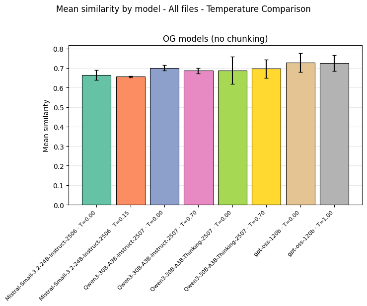
Temperature sensitivity analysis: scores remain flat across T=0 to T=0.70/1.00 for all tested models. Greedy decoding is optimal for extraction tasks.
The intuition is straightforward: extraction is not a creative task.
JSON structured output outperforms tool calling. For both promising models tested (Mistral-Small-3.2-24B and Qwen3.5-27B), JSON-constrained generation matched or outperformed tool calling. For Qwen3.5-27B, the gap was substantial (around 0.79 vs 0.70).
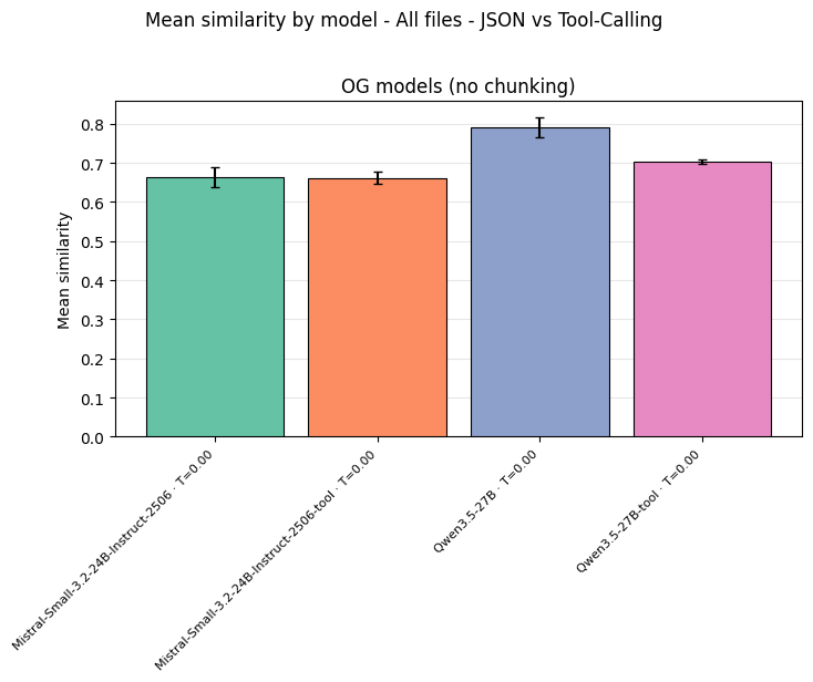
JSON structured output vs. tool calling: JSON matches or outperforms tool calling for both models tested. Tool calling adds parsing overhead with no accuracy benefit.
Tool calling introduces an additional parsing layer and model-specific formatting constraints with no accuracy benefit. JSON-constrained generation, where the inference engine constrains the output logits to produce valid JSON conforming to your schema, is the cleaner approach.
Thinking/reasoning mode does not help extraction. The thinking variant of Qwen3-30B showed no meaningful improvement over its base counterpart. Extended reasoning is valuable for problems requiring multi-step deduction; for extraction, the relevant information is in the document and the task is retrieval, not reasoning.
Consistency matters more than peak average. A key design goal of the CIEL project was to produce reliably reproducible results with consistently good quality, rather than optimising for the highest possible mean score at the cost of higher variance. A system that scores 0.78 on every run is more useful in production than one that averages 0.82 but occasionally drops to 0.60. This informed both model selection and the decision to use greedy decoding throughout.
MoE models exhibit higher score variance than dense models. Across the evaluation runs, Mixture-of-Experts architectures (Qwen3.5-35B-A3B, Qwen3.5-397B-A17B, GPT-OSS variants) showed noticeably wider confidence intervals on mean similarity scores compared to dense models of comparable effective parameter counts.
Fine-tuning on small datasets is unreliable. LoRA fine-tuning was explored on two models using 83 training samples. A 4B model responded positively (similarity score improved from around 0.54 to 0.64). A 20B model showed a marginal drop (around 0.70 to 0.68), likely because 83 samples provide insufficient signal-to-noise to shift a model of that size’s existing priors.
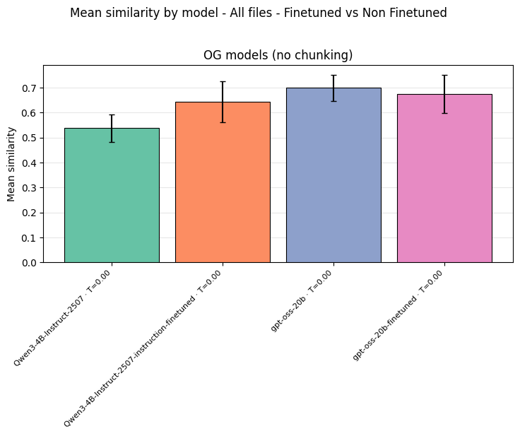
Fine-tuning results: the 4B model responds positively to LoRA adaptation; the 20B model does not, likely due to insufficient training data. Fine-tuning should be validated carefully, not assumed to help.
4. Infrastructure: Why Dedicated Inference, Not a Sovereign Token API
Per-token APIs deserve credit before the criticism because they are genuinely the right call for plenty of teams. There is nothing to commit to and no infrastructure to run and the cost only covers the tokens actually sent. When traffic goes quiet the bill goes quiet with it and there are no idle GPUs burning money overnight. It is also the quickest way to get something running and it soaks up spiky unpredictable load without anyone having to think about capacity. For prototyping or low or unpredictable volumes or any case where not babysitting a GPU fleet has real value, a token API is a perfectly sane default. The problems discussed below only really show up once a workload is running at steady production scale.
4.1 The problems with per-token pricing at scale
Prompt engineering inflates costs unpredictably. Structured extraction with few-shot examples means large system prompts. In the CIEL project, a typical extraction call had a system prompt of 30,000–35,000 tokens, as the few-shot examples alone dominated token usage. Under per-token pricing, every prompt engineering decision has a direct cost impact that is difficult to predict in advance.
No access to engine-level optimizations. The throughput gains available from KV cache quantization, prefix caching, and speculative decoding (see section 5 below) require control over the inference engine. A token API hides the engine entirely. We have been able to increase 2–3x throughput under parallel load.
Model stability cannot be delegated. The deprecation event described in the introduction is the concrete illustration. A shared API can retire, alter, or silently retrain a model at any time. A dedicated deployment pinned to a specific Hugging Face commit stays exactly as deployed until you choose to change it.
SLA and privacy guarantees are weak. Shared API providers typically offer no meaningful SLA for throughput or latency, and routing traffic through shared infrastructure makes strong privacy guarantees impossible regardless of jurisdiction. We have seen some strange gap in performance depending on context (peak hours in America) and it was impossible to debug/monitor it.
4.2 What a dedicated deployment looks like
Exoscale’s Concrete AI Dedicated Inference platform is a managed wrapper around vLLM running on dedicated GPU instances. The lifecycle is three operations:
model createregisters a Hugging Face model (public, gated, or private) and caches its weights on Exoscale’s infrastructure. Subsequent deployments load from cache, not from Hugging Face.deployment createprovisions a dedicated GPU instance, installs drivers, starts vLLM with your specified engine parameters, and exposes an OpenAI-compatible HTTPS endpoint with a private API key.deployment scaleadjusts replica count, including scaling to zero to pause GPU billing while preserving the endpoint URL and API key.
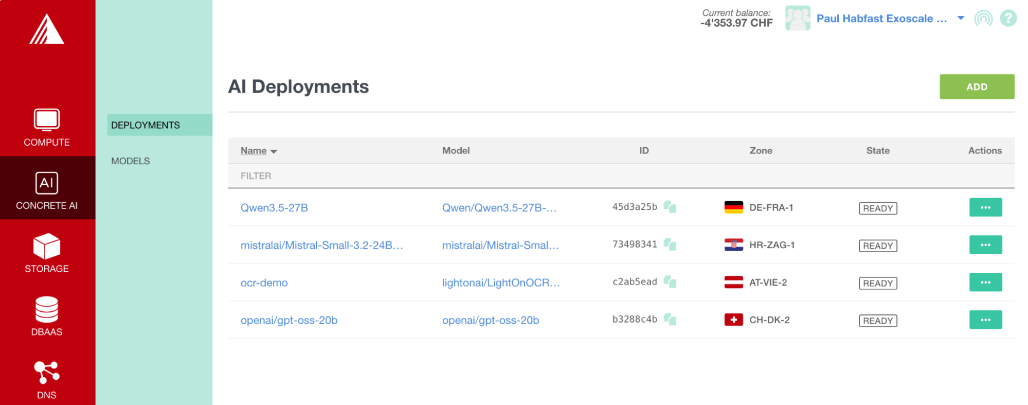
Exoscale Concrete AI portal: active model deployments across EU/CH zones. Each deployment runs on a dedicated GPU instance with a private, OpenAI-compatible endpoint.
The critical design decision: the endpoint is OpenAI-compatible. Code written against the openai SDK, LangChain, Instructor, or any comparable library works without modification. In the CIEL project, migrating the extraction pipeline from its GPT-4o integration to the LLM hosted on sovereign infrastructure was a configuration change and did not involve any code whatsoever.
Deployment zones available are all within EU/CH jurisdiction, with no third-country touchpoint at any stage of the pipeline.
5. Serving Configuration: Getting Production Performance from vLLM
Selecting the right model and deploying it on appropriate hardware is necessary but not sufficient. The gap between a naive vLLM deployment and a tuned one is significant, particularly for high-throughput batch workloads.
5.1 Understand your workload shape first
The CIEL extraction pipeline is representative of a class of workloads that differs importantly from interactive chat:
- High parallelism: a single document is split into many chunks and processed concurrently
- Large, shared system prompts: 30K+ tokens of few-shot examples, shared across all chunks from the same document type
- Structured output: JSON-constrained generation with a fixed schema
- Batch orientation: throughput matters more than time-to-first-token
This profile favours different optimizations than a low-latency chat endpoint. The goal is maximizing tokens processed per second across concurrent requests, not minimizing latency for any single one.
5.2 Key vLLM parameters
FP8 KV cache (--kv-cache-dtype=fp8)
The KV cache stores the key and value tensors produced during attention computation. Under high concurrency, it is the dominant consumer of GPU memory. Storing these tensors in FP8 (8-bit) rather than BF16 (16-bit) halves the cache memory footprint, which directly enables larger batch sizes and longer effective context windows without exceeding VRAM limits. Be aware that this is not entirely free. Moving from 16 bits to 8 rounds each stored value slightly and introduces a small error on every token. On a short prompt this error is negligible but over a long context it accumulates as the model relies on thousands of these values at once and the small errors begin to compound. This is why FP8 KV cache quantization can affect output quality on long inputs first, and why some models tolerate it better than others depending on their sensitivity to the loss of precision. In our testing, output quality was not affected by the KV cache quantization. Other use cases may not so this should be validated on the target workload before being relied upon in production.
Prefix caching (--enable-prefix-caching)
When many requests share a long common prefix, prefix caching avoids recomputing the attention keys and values for the shared prefix on every request. For workloads with 30K+ token system prompts, this can dramatically reduce effective compute per request. This would tend to also be true of coding agent applications.
Context window sizing (--max-model-len=80000)
Do not simply set this to the model’s maximum (often 128K–262K). Every request’s KV cache allocation is bounded by this value, which directly affects how many concurrent requests can fit in memory. Measure your actual maximum context usage (system prompt + largest document chunk + expected output + retry overhead) and set the window to match, with reasonable headroom.
In the CIEL project, real-world measurements showed that 80K tokens was sufficient to cover the largest observed calls (system prompt ≈32K + document ≈5K + output ≈500 + retry overhead), while leaving meaningful room for batch parallelism.
Speculative decoding
LLM inference is fundamentally sequential: each token requires a full forward pass. Speculative decoding breaks this by having a fast “draft” mechanism propose several candidate tokens ahead of time, which the main model verifies in a single parallel pass. If the candidates are accepted, multiple tokens are committed in one step; if rejected, the model falls back to standard generation. Crucially the output is identical to standard greedy decoding, speculative decoding is a pure throughput optimization with no quality trade-off.
5.3 GPU selection
For the models that performed best in evaluation:
| Model | Architecture | Est. VRAM (BF16) | Fits on |
|---|---|---|---|
| Qwen3.5-27B | Dense | 54 GB | RTX Pro 6000 (96 GB) |
| Mistral-Small-3.2-24B | Dense | 48 GB | RTX Pro 6000 (96 GB) |
| Qwen3.5-35B-A3B | MoE (3B active) | 70 GB total | RTX Pro 6000 (96 GB) |
| Qwen3.5-397B-A17B | MoE (17B active) | 794 GB total | Multi-GPU or larger instance |
For MoE models, the distinction between total and active parameters matters for accuracy estimation, but VRAM sizing must account for total parameters: all weights must be loaded even if only a fraction are active per forward pass.
The RTX Pro 6000 with 96 GB VRAM comfortably serves the 27B dense and 35B MoE models with room for KV cache and parallel batch headroom, which makes it a sweet spot for this class of workload.
6. Handling Long Documents: Structure-Aware Chunking and Merging
In many domains such as legal, real estate or engineering, most real-world documents exceed comfortable context windows. The chunking strategy in the CIEL project originated as a response to a hard technical constraint: early in the project, the open-weight models under consideration had relatively small context windows, making full-document processing simply impossible for longer inputs.
What happened in practice was more interesting: chunking turned out to deliver precision and throughput gains beyond just working around context limits. Smaller, focused fragments reduce the amount of irrelevant context the model must attend to, which improves extraction precision for dense or complex content. They also enable parallel processing across chunks, which improves throughput significantly for long documents.
The relationship between chunking and model capability has also evolved. The newer ones like Qwen3.5 and Mistral-Small-3.2 handle long contexts well so there is no need to chunk nearly as much as before. How small the chunks should be really depends on which model is running. Older or smaller models do better with tight chunks while newer ones hold their precision across much larger ones and there is no reason to slice them up the same way. Chunk size should be picked for the model actually being deployed and not for the one the strategy was first designed around.
6.1 Segment on structure, not on character count
Documents like contracts and quotes have strong internal structure: numbered sections, headings, tables, annexes. These boundaries carry semantic meaning that a fixed-token split will frequently cut across.
A more effective approach detects section boundaries from typographical and linguistic cues: numbered headings (including Markdown-style ## headers and plain 2.3.4 Title patterns), all-caps section markers, multilingual chapter/section/article/annex labels, and table-embedded section identifiers. One important refinement: headers that appear more than twice with identical wording are treated as repeated page headers, not section boundaries, and excluded from the split point candidates.
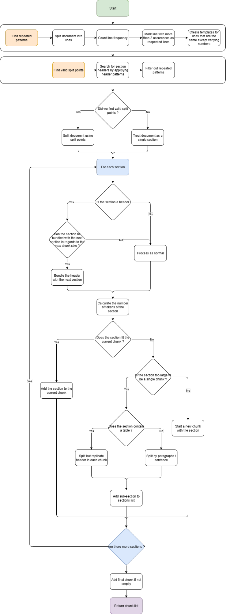
Structure-aware segmentation algorithm: the first stage identifies valid split points based on typographical markers; the second stage packages sections into fragments that respect the LLM’s context limit while preserving structural coherence.
Tables receive special handling. They often carry the quantitative data most critical to extraction (line items, pricing, quantities). When a table must be split across chunks, the header row is duplicated into each chunk so that every fragment remains interpretable by the model in isolation.
6.2 Merge partial extractions by completeness score
Each chunk is processed independently by the LLM, producing a partial structured output. These need to be combined into a single document-level structure without requiring cross-chunk reasoning from the model.
A score-based approach works well: assign each extracted object a completeness score based on the proportion of populated fields. When multiple chunks produce extractions for the same object, retain the version with the higher completeness score. For list-type objects (line items, contracting parties), combine elements from all chunks and deduplicate. When no explicit identifier is available for deduplication, derive a temporary one from stable attributes (name + address, for example).
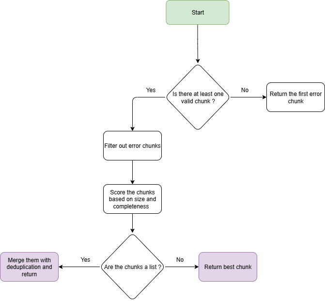
Score-based merging: fragment-level extractions are scored by completeness and merged without requiring the model to reason across chunk boundaries.
6.3 Quantifying the chunking trade-off
Chunking introduces a measurable but acceptable accuracy penalty. In evaluation, no-chunking consistently outperformed chunking by roughly 0.05–0.10 similarity score for both tested models:
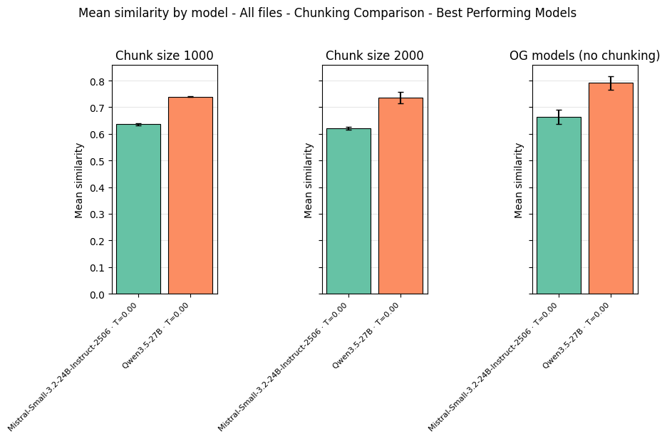
Chunking strategy comparison: no-chunking yields the best scores for both models, but chunking remains viable for documents exceeding the context window. The performance gap narrows at chunk size 2000.
The practical implication: for documents within your context window, process them whole. For documents that exceed it, chunking is a viable fallback with a known and bounded quality cost. Tune chunk size based on both input and expected output density; when output tokens are high (e.g., extracting many line items), smaller chunks with more focused extraction outperform larger chunks where the model may lose track of the output structure.
7. The Orchestration Layer: Making an LLM Behave Deterministically
An LLM without orchestration is not a production system. It will occasionally omit required fields, return invalid JSON, fail on edge cases, or produce different outputs for identical inputs. The orchestration layer is the engineering that converts probabilistic model behaviour into a reliable, reproducible extraction pipeline.
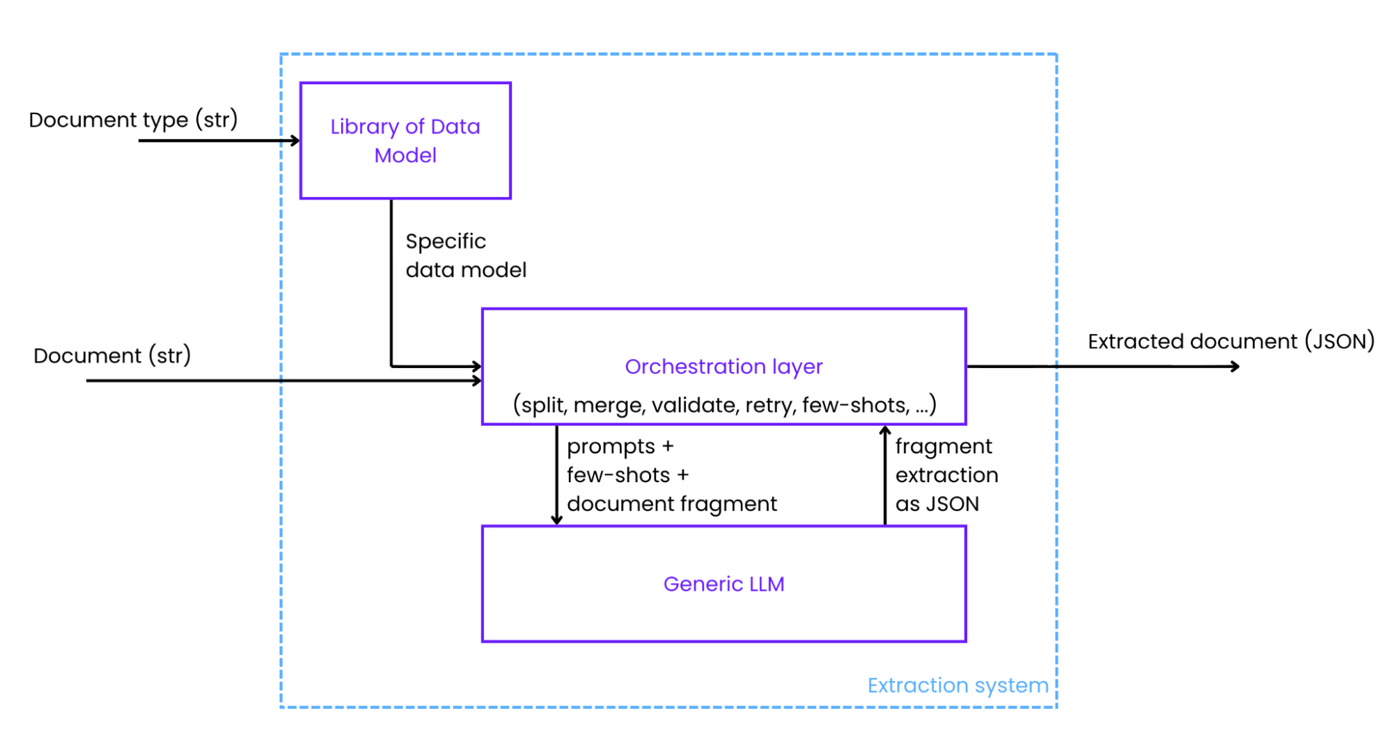
Extraction system architecture: the orchestration layer wraps the LLM with schema enforcement, retry logic, and fragment merging, producing a deterministic structured output from an adaptive model.
Three components do most of the work:
Schema enforcement (Pydantic). Define your target output as a typed Python class: fields, types, nested structures, required vs. optional attributes. Every LLM response is validated against this schema before it is accepted. Validation failures produce structured error messages that feed directly into retry logic.
Prompt and retry management (Instructor). Wraps the LLM call with automatic retry on validation failure: if Pydantic rejects the output, Instructor reformats the prompt (adding the error message, adjusting examples, or reducing scope) and retries. Every attempt is logged and the retry budget is bounded, so the pipeline terminates predictably even on pathological inputs.
Observability (Phoenix or equivalent). Traces every LLM call with its full context: system prompt, user prompt, raw output, token counts, latency, retry history. It lets you answer questions like “why did this document fail?” or “which document types are consuming the most tokens?”. It is also how you will discover that your system prompt has grown to 32K tokens over successive iterations of few-shot example additions, which may be surprisingly easy to lose track of.
Few-shot examples are the primary mechanism for specializing a general-purpose LLM to your extraction task without fine-tuning. Include 2–4 input/output pairs per document type, covering common structures and known edge cases. Keep them in version control. Update them when the schema changes. The few-shot examples are, in effect, the specification that the model follows.
8. Migration Checklist
A condensed, actionable summary of the steps above:
Before you migrate:
- Instrument your existing pipeline with an observability tool; collect baseline token counts, latency, and retry rates
- Build an evaluation set: 50+ examples with ground-truth structured outputs, covering your full distribution of document types and edge cases
- Audit your prompt structure: measure actual system prompt size, few-shot count, and output schema complexity
Model selection:
- Shortlist 8–12 open-weight candidates based on VRAM fit, license, and release date, or other hard requirements such as supported languages.
- Run zero-shot, T=0, JSON output benchmarks across all candidates on your evaluation set
- Compare JSON structured output vs. tool calling on your top 3–4 candidates
- Confirm VRAM fit with realistic batch sizes (total parameters × 2 GB for BF16, then add KV cache headroom)
- Consider fine-tuning only after establishing a strong zero-shot baseline, and only with a held-out validation split
Infrastructure:
- Choose deployment zone for your data residency requirements
- Configure vLLM: fp8 KV cache, prefix caching, context window sized to actual workload
- Select speculative decoding strategy (native MTP head if available; n-gram lookup otherwise)
- Verify that your existing client code works against the OpenAI-compatible endpoint with only URL and API key changes
After migration:
- Re-run the full evaluation set on the new stack and compare to your commercial baseline
- Set up alerts on retry rate and p95 latency
- Pin your model to a specific commit; treat upgrades as deployments, not automatic updates
- Document your vLLM configuration alongside your model selection rationale
9. What Sovereign Infrastructure Actually Costs and Buys
Hosting an LLM on sovereign infrastructure is not free. Relative to a pay-per-token commercial API, it requires:
- Upfront investment in model evaluation. You need to know which model to deploy before you deploy it, and that requires running your own benchmarks.
- An evaluation set. Building it requires collecting documents, producing ground-truth extractions, validating them with domain knowledge.
- Operational responsibility. You own the inference stack. Model updates, vLLM version upgrades, and capacity planning are your team’s concern.
- Slightly more engineering. Tuning for throughput under parallel load requires understanding vLLM’s parameters and your workload’s profile.
What you get in return:
- No surprise deprecations. The model you deploy is the model that runs until you decide to change it.
- Predictable costs. GPU-hour billing decouples cost from prompt verbosity and output complexity. You don’t pay extra for a large system prompt or for increased data volume, as long as you remain within the operational limits of the reserved instances. This enables new/more use cases to use the card without thinking about the price per token, such as more tests, experiments, etc.
- Full control over model version and engine configuration. You can enable and tune optimizations that are simply not accessible through a token API.
- Compliance confidence. For regulated industries, the infrastructure sovereignty chain is end-to-end and documentable: data processing, cached model weights, and inference compute all within a single European legal jurisdiction, under a contract governed by European law.
- Autonomy and independence. Since the model is open-weight and is run on opensource software, there’s no vendor lock-in and migrating to another provider or even private infrastructure is completely feasible.
And, in the CIEL project’s case: better accuracy than the commercial baseline. This was a clear target but going in it wasn’t a guaranteed outcome. It is a consequence of the evaluation-driven approach described throughout this post.
Acknowledgements
CIEL was a team effort across four organisations. With thanks to:
- Recarta: Géraud de Laval and Étienne Friedli, who led the data modelling, orchestration design, and production integration.
- HEIG-VD / IICT: Teo Ferrari and Andrei Popescu-Belis, who designed and built the long-document algorithms and the evaluation framework.
- SDSC: Clément Lefebvre, who ran model evaluation, benchmarking, and vLLM configuration.
- Exoscale: Paul Habfast, who designed and built the Concrete AI Dedicated Inference platform and led the production deployment.
The project was funded by SEAL Innovation and the Service de la promotion de l’économie et de l’innovation (SPEI) of the Canton de Vaud, under the Programme d’innovation EPFL·HEIG-VD·UNIL.

