Inside an LLM: From Prompt to Tokens
 Luc Juggery
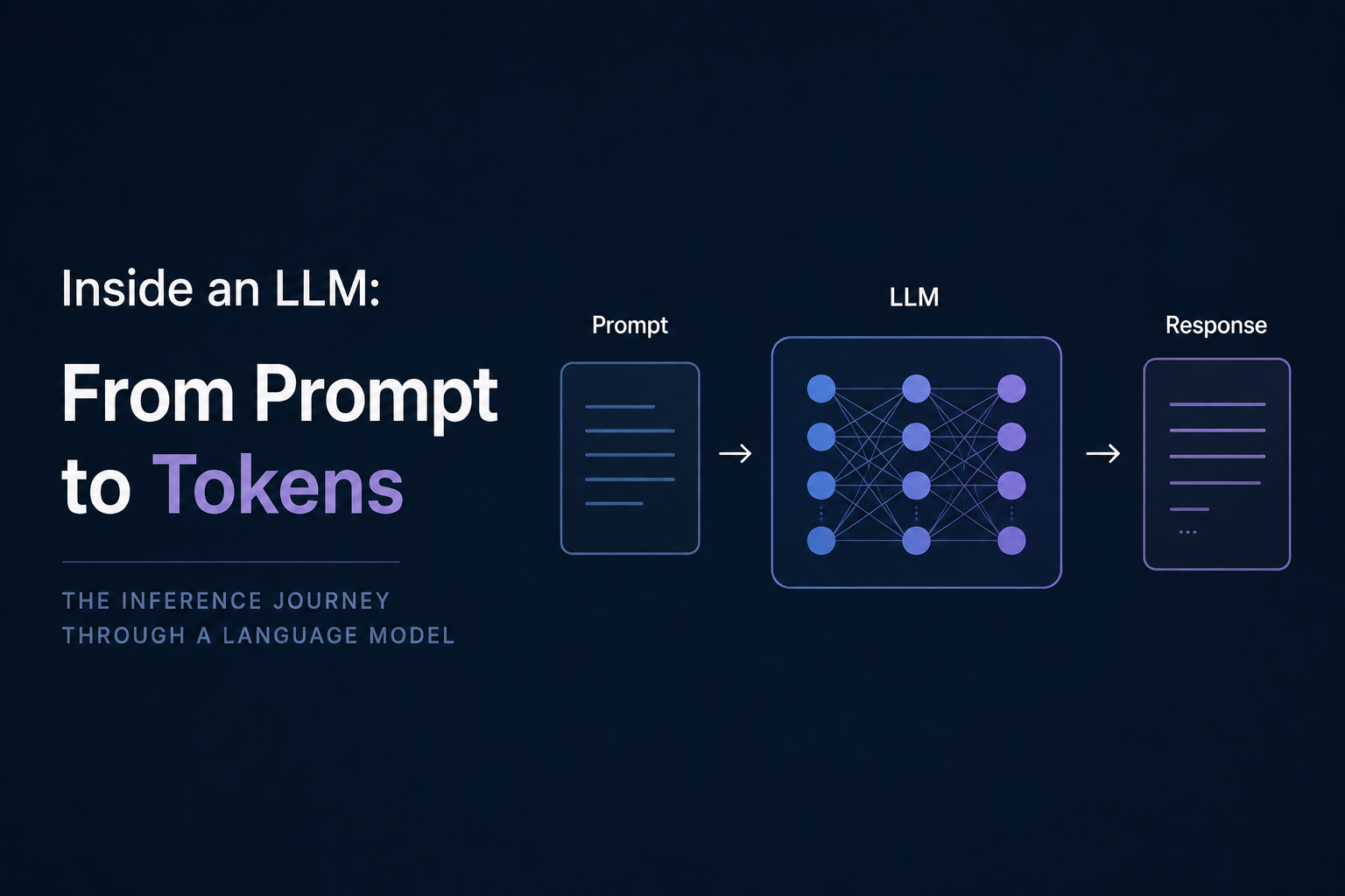
LLM inference is the process of transforming a prompt into generated tokens. This article explores what happens inside the model during that journey, covering prefill and decode, hidden states, attention, MLP layers, and the KV cache. It does not cover advanced inference engineering topics.
Quick summary of this article
- Understand how LLM inference transforms a prompt into generated tokens
- Learn the difference between prefill and decode, and follow the forward pass through transformer layers
- Discover how attention, MLPs, and hidden states progressively refine a token’s representation
- Explore the role of the KV cache and inspect the real tensors that make up an LLM
Prefill and Decode: The Two Phases of Inference
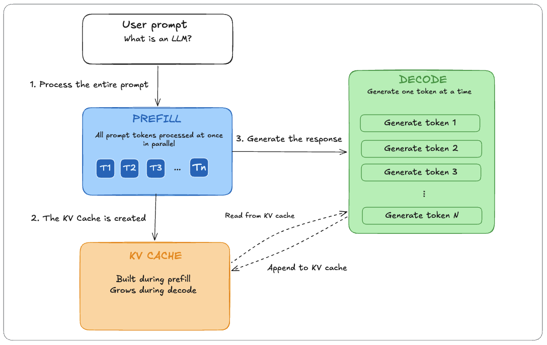
First, comes the prefill phase, during which all prompt tokens are passed through the model. Their hidden states are computed, and their K/V tensors are stored in the KV cache.
We’ll dive in the hidden state and KV Cache later in this article. For now you can think of:
- the hidden state as the continuously evolving representation of a token
- the KV Cache as a memory that lets the model avoid repeating work
After the prefill phase, the model enters the decode phase, where it generates one new token at a time.
Looking at both steps:
prefill | decode | |
|---|---|---|
| Input | Entire prompt at once | One token at a time |
| Parallelism | Full: all tokens in parallel | Sequential within a sequence |
| ** Typical bottleneck** | Often compute-bound | Often memory-bandwidth-bound |
| Output | Populated KV cache and next-token prediction | One generated token per step |
To understand what happens during inference, we first need to understand the forward pass.
The Core Operation: The Forward Pass
Both prefill and decode execute the same computation: the forward pass, which is the journey from an input token to a prediction for the next token.
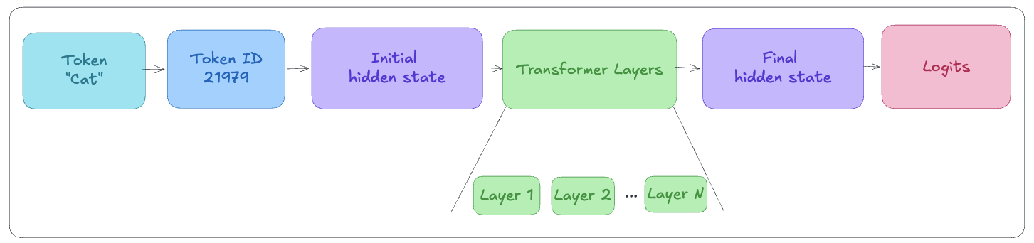
Before the forward pass, the input text is converted into numerical token IDs.
That token ID is then used as an index into the embedding table W_E. The selected row becomes the token’s embedding vector. This embedding is also the token’s initial hidden state.
W_E is a large lookup table containing one row per token in the model’s vocabulary (set of all the tokens the model knows). Looking up a token ID means selecting the corresponding row.After this point, the model no longer works with token IDs. Everything flowing through the network is a hidden state: a vector representing the model’s current understanding of the token.
That hidden state then passes through a series of transformer layers, each one refining it. At the end, the final hidden state is projected into a score for every possible next token. These scores are called logits, and the next token is sampled from them.
The following sections explain what happens inside each transformer layer.
How a Transformer Layer Refines a Hidden State
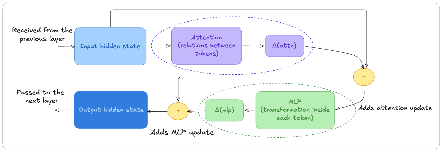
A transformer layer contains two major components:
- Attention, which allows tokens to retrieve information
- MLP, which transforms each token independently
Attention and the MLP each produce an update that is added directly to the hidden state.
The hidden state always has the same size throughout the network. This size is usually called d_model. For instance, for Llama 3 8B, d_model = 4096, meaning every token is represented by a vector of 4096 floating-point values.
Attention computes an update Δ(attn) and the MLP computes another update Δ(mlp). Both are added directly to the hidden state.
The hidden state of each token accumulates information during its journey across all the transformer layers of the model.
Let’s now have a closer look at the attention mechanism.
Attention: How Tokens Communicate
The purpose of attention is to allow tokens to retrieve useful information from other tokens in the context.
Consider the sentence:
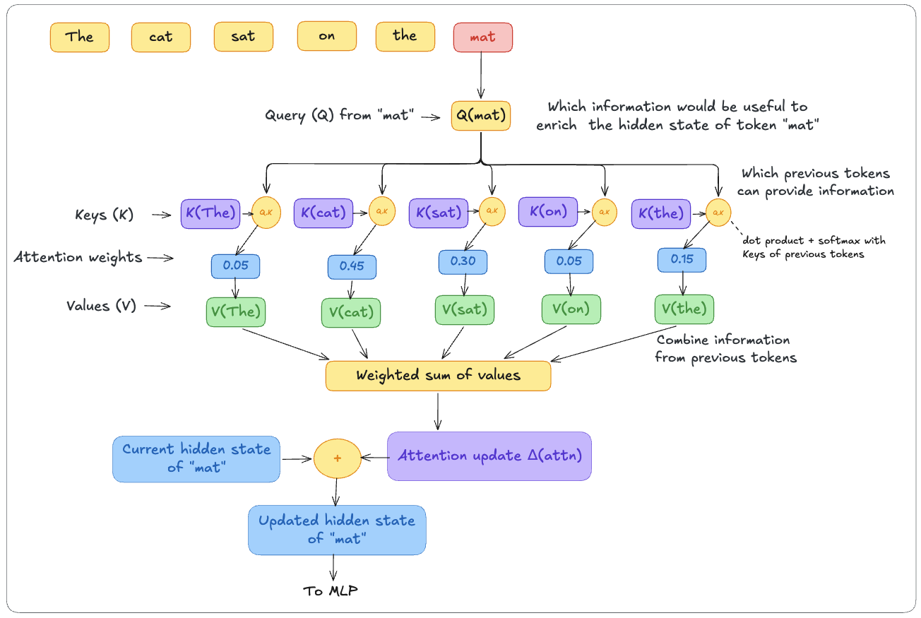
The cat sat on the matWhen the model processes “mat”, its hidden state needs context from earlier tokens: what is the subject? What action is performed?
To find that context, the hidden state is projected through three different learned matrices, each producing a different vector:
- one that determines what information is needed (Q)
- one that determines how the token can be matched (K)
- one that determines what information it can contribute (V)
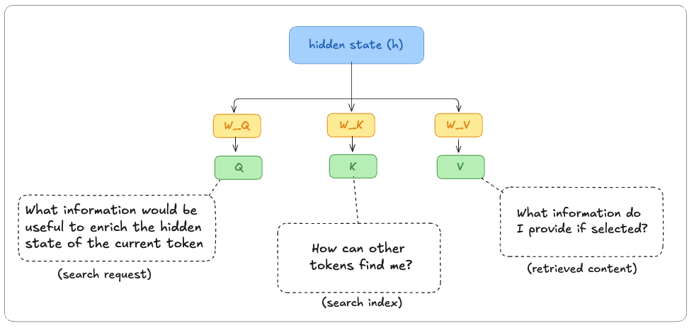
- Q represents what information would be useful for this token at this layer. You can think of it as a search request generated from the token’s current hidden state. For “mat”, that request may focus on information such as the subject (“cat”) or the action (“sat”), although it is encoded as a vector rather than a human-readable question.
- K is a label derived from a token’s current hidden state and exposed for matching. The Q of “mat” is compared against the K of every other token (“The”, “cat”, “sat”, “on”, “the”) to produce a relevance score.
- V carries the actual information a token contributes once selected. The V vectors are weighted by those scores and summed to produce the attention output.
This produces an attention update Δ(attn) that is added directly to the hidden state.
W_O, projects the combined attention output back to d_model, so it can continue through the network.Multi-head Attention
In practice, attention is performed multiple times in parallel, so each attention head can learn a different type of relationship:
- subject ↔ verb
- pronoun references
- word order
- semantic associations
The outputs of all heads are concatenated and projected through W_O.
MLP: How Tokens Think
If attention is how tokens communicate, the MLP is how they think.
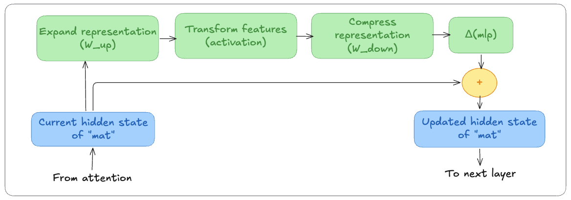
The MLP operates only on the current token’s hidden state. Its purpose is to refine that representation and extract more useful features from it.
The MLP performs three main steps:
- Expand the hidden state into a larger internal dimension (using
W_up) - Apply a gating mechanism:
W_gatelearns which parts of the expanded representation are important and suppresses the rest - Compress back to
d_model(usingW_down)
By temporarily expanding into a larger internal space, the model can perform more complex transformations than would be possible directly in d_model.
The result is another update: Δ(mlp), which is added directly to the hidden state.
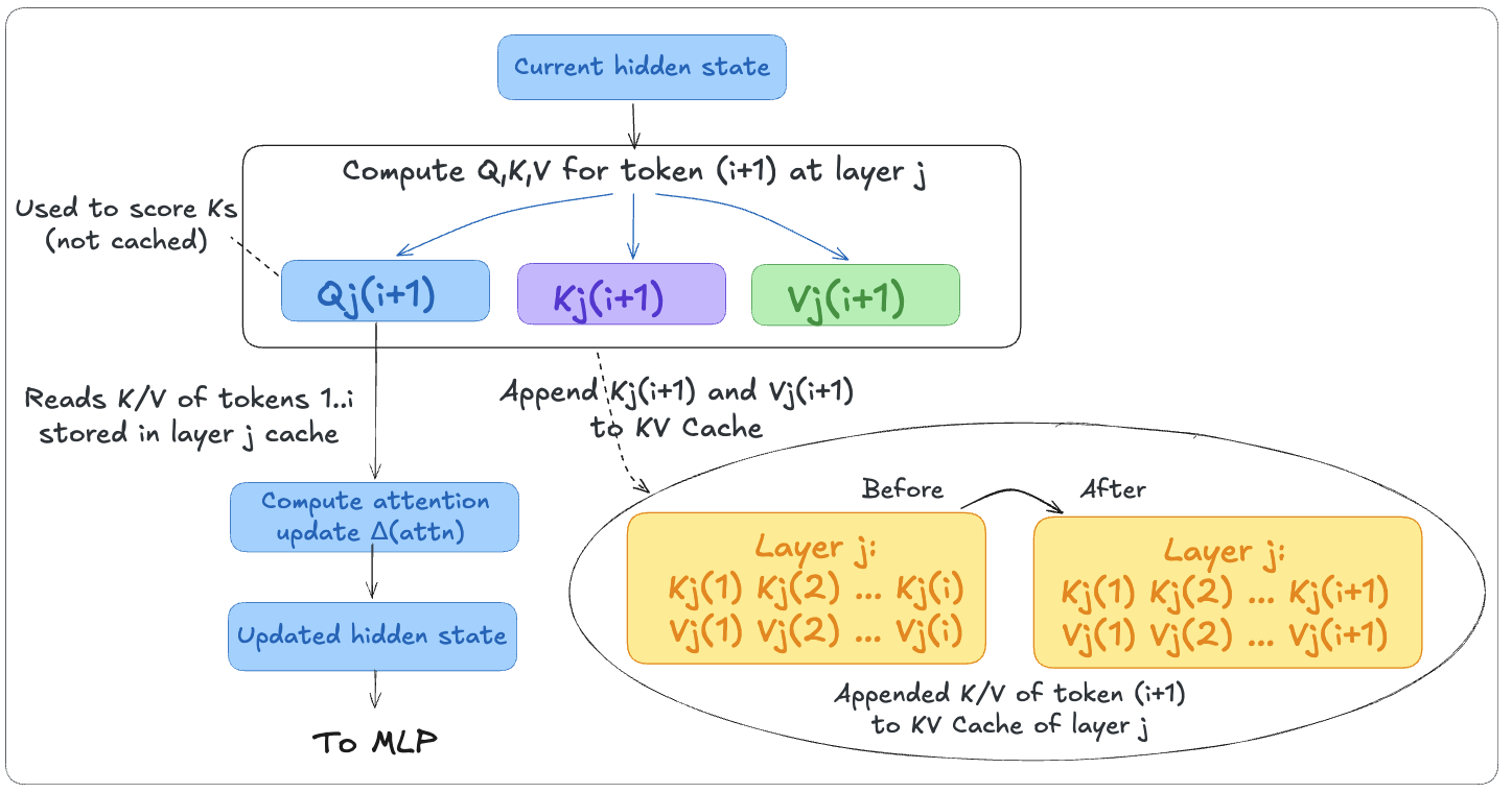
The KV Cache
Without a cache, the model would recompute keys and values for every previous token on each generation step. For a long prompt, that is a lot of redundant work.
Instead, K and V tensors are stored the first time they are computed and reused throughout decode. Q is never cached as it only makes sense for the current token, and it’s discarded after use.
During prefill, the cache is populated: every prompt token gets one K and one V vector at every transformer layer.
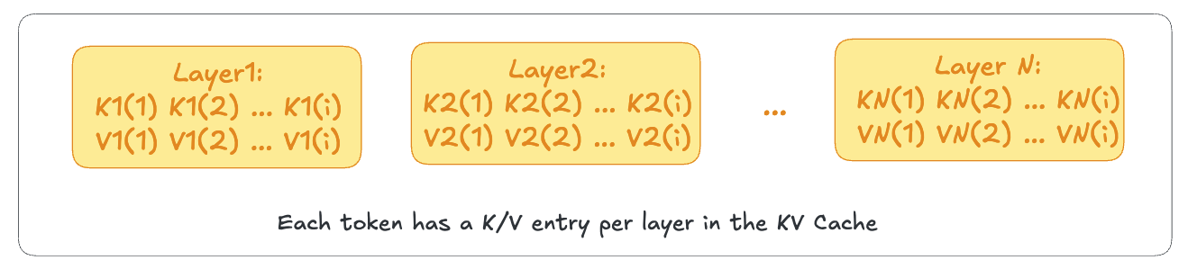
During decode, every newly generated token appends its own K/V pair to every layer’s cache. The cache grows by one entry per layer with each new token.
For large models and long contexts, KV cache memory can easily reach several gigabytes and becomes one of the main bottlenecks for inference.
The Tensors Behind an LLM
For reference, each layer contains the following tensors (they may not have the exact same names though).
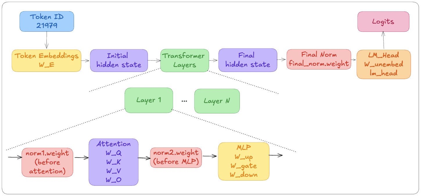
The diagram includes tensors that were not covered earlier:
- norm1.weight, norm2.weight, and final_norm.weight belong to RMSNorm layers, which help keep hidden-state values in a stable numerical range
- W_unembed (often called lm_head) converts the final hidden state into logits, one score for every token in the vocabulary
Inspecting a Real Model
Everything above can be verified on a real model. The example below uses SmolLM2-135M, a small openly available model that follows the same Llama-style architecture. No HuggingFace account needed.
pip install torch safetensors huggingface_hub

# Download the model. With recent versions of huggingface_hub:
hf download HuggingFaceTB/SmolLM2-135M --local-dir ./smollm
# Older versions: huggingface-cli download HuggingFaceTB/SmolLM2-135M --local-dir ./smollmimport re
from safetensors import safe_open
def natural_key(s):
return [int(t) if t.isdigit() else t for t in re.split(r'(\d+)', s)]
with safe_open("./smollm/model.safetensors", framework="pt") as f:
for key in sorted(f.keys(), key=natural_key):
shape = f.get_slice(key).get_shape()
print(f"{key:55s} {shape}")This reads shapes directly from the file header without loading the weights into memory.
See full output
$ python inspect_tensors.py
model.embed_tokens.weight                               [49152, 576]
model.layers.0.input_layernorm.weight                   [576]
model.layers.0.mlp.down_proj.weight                     [576, 1536]
model.layers.0.mlp.gate_proj.weight                     [1536, 576]
model.layers.0.mlp.up_proj.weight                       [1536, 576]
model.layers.0.post_attention_layernorm.weight          [576]
model.layers.0.self_attn.k_proj.weight                  [192, 576]
model.layers.0.self_attn.o_proj.weight                  [576, 576]
model.layers.0.self_attn.q_proj.weight                  [576, 576]
model.layers.0.self_attn.v_proj.weight                  [192, 576]

... (layers 1–28 have identical structure) ...

model.layers.29.input_layernorm.weight                  [576]
model.layers.29.mlp.down_proj.weight                    [576, 1536]
model.layers.29.mlp.gate_proj.weight                    [1536, 576]
model.layers.29.mlp.up_proj.weight                      [1536, 576]
model.layers.29.post_attention_layernorm.weight         [576]
model.layers.29.self_attn.k_proj.weight                 [192, 576]
model.layers.29.self_attn.o_proj.weight                 [576, 576]
model.layers.29.self_attn.q_proj.weight                 [576, 576]
model.layers.29.self_attn.v_proj.weight                 [192, 576]
model.norm.weight                                       [576]
You can map every row back to the concepts introduced earlier: q_proj is W_Q, k_proj is W_K, v_proj is W_V, o_proj is W_O, and the MLP contains up_proj, gate_proj, and down_proj.
The attention, MLP, embeddings, and normalization layers discussed in this article are implemented as learned tensors stored in the model file. Inspecting a real model lets you see those tensors directly.
Putting It All Together
During inference, every token follows the same path:
- The token ID is looked up in
W_Eto produce the initial hidden state - Each transformer layer refines that hidden state: attention pulls in context from other tokens and the MLP transforms the representation internally
- The final hidden state is projected into
logits, which are converted into probabilities. The next token is then selected from those probabilities
From a high level view, inference is the repeated transformation of hidden states. The weights stored in the model define how those transformations happen, while the KV cache stores information that allows the model to avoid recomputing work it has already performed.

